MPC3S toolbox

---

Description

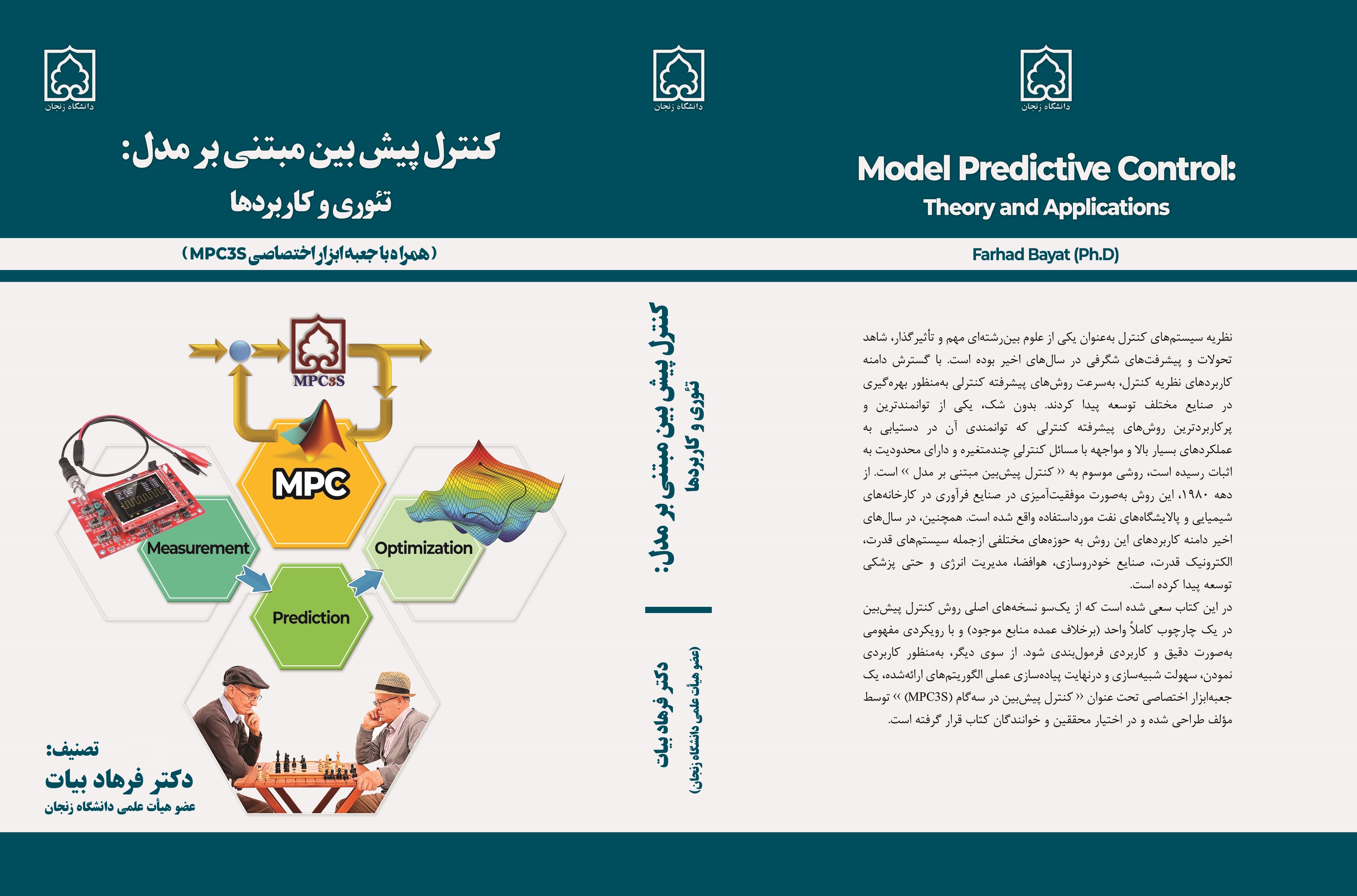
MPC3S is an open-source toolbox that provides several functions to Define, Solve, and Simulate different variations of the linear model predictive control (MPC) approach.

>>  Download User Guide for MPC3S  <<

(Currently, it is available just in PERSIAN)

(English version will be available soon)

Videos for learning MPC3S toolbox in YouTube:

---

System Requirements

The MPC3S toolbox supports all the following platforms:

• Windows 32bit/64bit
• Linux 32bit/64bit,
• Mac 32bit/64bit,
• MATLAB online.

---

Installation

• For Installation:   
  1. Download MPC3S toolbox according to your operating system:
     • Win 64-bit-32-bit  (NEW Version 6.0)
       • Linux 64-bit  (Version 5.0)
       • Linux 32-bit  (Version 5.0)
         • Mac 64-bit  (Version 5.0)
         • Mac 32-bit  (Version 5.0)
  2. Unpack and Run the "MPC3S_install.m" file inside the toolbox folder.
  3. You are done. :)

---

Features

• Unlike most existing MPC toolboxes, the MPC3S can handle several models including FIR, FSR, CARIMA, and State-Space (SS) in a unified framework.
• The MPC3S toolbox easily lets you specify plant and disturbance models, horizons, constraints, weights, filters for measurement noise reduction, and observer model (in SS model).

• Any MPC problem can be done in just 3 steps:

• Step-1: Define your own MPC problem just by calling a single function "MPC_Problem()".
• Step-2: Solve your defined MPC problem just by calling a single function "MPC_Solve()".
• Step-3: Simulate the designed MPC problem just by calling a single function "MPC_Sim()".

• For practical applications, the MPC3S toolbox provides deployable optimization solvers and also enables you to use custom solvers.
   
• To control a nonlinear plant, you can first linearize the plant model and design a linear MPC using the MPC3S toolbox for the linear system and then performing the closed-loop simulation with the nonlinear plant model in the loop.
   
• For applications with fast dynamics, or in any case, you would not like to embedded optimization solvers, the MPC3S toolbox lets you generate an Explicit Model Predictive Controller (EMPC) just by calling a single function "MPC_TO_EMPC()".

---

A Simple Example:

Consider a 1-st order SISO system with the following state-space model (Ts=1 sec):

The cost function associated with the MPC problem is assumed as:

where the design parameters are chosen as:

Furthermore, the following constraints are assumed:

We aim to design an MPC law for this system, and simulate the closed loop system with the following parameters:

SOLUTION:

Step-1:

Problem = MPC_Problem('SS');

Problem.Plant.Model.A = 0.5;

Problem.Plant.Model.B = 1;

Problem.Plant.Model.C = 1;

Problem.Plant.Ts = 1;

Problem.Plant.ny = 1;

Problem.Plant.nu = 1;

Problem.Cost.Np = 10;

Problem.Cost.Nc = 5;

Problem.Cost.Gama = 2;

Problem.Cost.Lamda = 1;

Problem.Constraints.umax = 1;

Problem.Constraints.umin = -1;

Problem.Constraints.Dumax = 0.2;

Problem.Constraints.Dumin = -0.2;

Step-2:

mpcLaw = MPC_Solve(Problem);

Step-3:

SimParams = MPC_SimParams('SS');

SimParams.Ref = 2*ones(1,50);

SimParams.Dist = [zeros(1,20),0.5*ones(1,30)];

SimParams.Noise.y = [zeros(1,30),0.05*(2*rand(1,20)-1)];

Results= MPC_Sim(mpcLaw,SimParams);

MPC_Plot(Results)

NOTE:

Two auxiliary functions "MPC_SimParams()" and "MPC_Plot()" are utilized to prepare simulation parameters and plotting the simulation results, respectively.

Finally, the closed-loop simulation results are shown in Figure 1 that verify the design objectives.

Figure 1: Closed-loop simulation results.